CosyVoice3 的训练代码已经开源,这次最核心的变化在于 Flow Matching 模块从 U-Net 升级为 DiT(Diffusion Transformer)架构。本文以 cosyvoice/flow 目录下的最新代码为切入点,结合配置文件 cosyvoice3.yaml,从模型架构、Flow Matching 原理、条件信息输入机制、流式推理设计等维度对 DiT 模块进行解读。由于 DiT 的实现复用了 CosyVoice 1 和 CosyVoice2 中的不少关于 CFM 的基础代码,本文也一并进行简要分析。
1. 整体架构概览
CosyVoice 系列的语音合成模型分为三个模块:LLM→Flow Matching→HiFiGAN(HiFTNet),其中 Flow Matching(后文有可能简称为 CFM) 模块负责将离散的 speech token 转化为连续的梅尔特征,因为 HiFiGAN 声码器技术已经相对成熟且效果不错,所以合成音频的音色、音质基本上可以认为是 Flow Matching 这个模型来保证的。本文基本不涉及 Flow Matching 的基础理论,主要关注 CosyVoice 里的具体代码实现。
在 CosyVoice 开源代码下,Flow Matching 模块的顶层类为 CausalMaskedDiffWithDiT(定义于 cosyvoice/flow/flow.py),其内部结构如下:
1 | CausalMaskedDiffWithDiT |
与 CosyVoice 前代模型的架构变化
| 版本 | flow 类 | 编码器 | 上采样方式 | 去噪网络 |
|---|---|---|---|---|
| v1 | MaskedDiffWithXvec |
ConformerEncoder + LengthRegulator | 线性插值 | U-Net |
| v2 | CausalMaskedDiffWithXvec |
UpsampleConformerEncoder | 转置卷积 + Conformer | U-Net |
| v3 | CausalMaskedDiffWithDiT |
PreLookaheadLayer | repeat_interleave |
DiT |
可以看出,CosyVoice3 的核心变化是:用轻量 PreLookaheadLayer 替代了 Conformer Encoder,用 DiT 替代了 U-Net,将模型参数集中到 Transformer 网络上。
2. 模型结构解读
本章按照模型从输入到输出的数据流向,依次介绍输入信息、注入模型的方式,token 编码与上采样、DiT 网络结构,训练目标和推理采样方式。
2.1 输入条件与信息融合
DiT 在推理/训练时一共接收五路信息,它们的注入方式和生命周期存在一些差异:
| 参数名 | 信息 | 注入方式 | 注入位置 | 随 ODE 迭代变化 |
|---|---|---|---|---|
| mu(token emb) | speech token 信息 | concat → Linear | DiT 输入 | 不变 |
| spks(speaker) | 说话人表征 | concat → Linear | DiT 输入 | 不变 |
| cond(prompt mel) | 参考 prompt mel | concat → Linear | DiT 输入 | 不变 |
| x(噪声/状态) | ODE 当前状态 | concat → Linear | DiT 输入 | 每步更新 |
| t | 时间步 | AdaLN-Zero 调制 | DiT 每一层 | 从0到1递增 |
上述信息进入网络,主要通过:
- 方式一:concat 投影,mu / spks / cond / x 在入口
InputEmbedding中拼接为 320 维后线性投影到 1024 维,之后仅通过 attention 间接影响各层。 - 方式二:AdaLN-Zero 调制,时间步 t 在每一层通过 6 个调制参数(shift/scale/gate × attn/FFN),能够在每个深度上调制影响模型能力,后文会详细讲解。
DiT 通过 InputEmbedding 层(定义于 cosyvoice/flow/DiT/dit.py)将四路信号在入口处融合:
1 | class InputEmbedding(nn.Module): |
拼接维度:80(噪声x) + 80(prompt mel) + 80(speech token embedding) + 80(说话人spk embedding) = 320 → Linear → 1024。
2.2 Prompt 训练/推理设计
CosyVoice 从 v1 到 v3 一直沿用相同的 prompt 条件设计,核心目的是让 Flow Matching 模型具备 in-context 能力:给定一段参考音频(prompt),生成与之音色、风格、音质一致的新语音。
2.2.1 训练阶段
训练时(cosyvoice/flow/flow.py 的 forward 方法),完整的 token 序列直接从 batch 中读入,不做任何 prompt / 非 prompt 的拆分或拼接。”prompt” 的概念仅通过条件变量 cond 体现,即随机选取序列前缀的一段 mel 帧作为条件输入:
1 | conds = torch.zeros(feat.shape) |
DiT 的输入 y(即 noised mel)覆盖全序列,cond 作为额外条件信号与 y 一起 concat 输入 DiT。训练 loss 同样在全序列上计算(包含 prompt 区),prompt 区的梯度参与反向传播,使模型学会利用 prompt cond 中的参考信息来合成更好的效果。
针对 prompt 部分,
cond中包含 ground-truth mel 并不构成信息泄露:模型的预测目标是速度场u = x₁ - (1 - σ_min) · z(其中x₁是真实梅尔),而非直接复原 mel 本身。即使cond提供了参考 mel,模型仍需从带噪状态y出发预测正确的速度方向。简而言之,cond的作用是提供风格/音色参考,而非直接给出答案。
2.2.2 推理阶段
推理时(inference 方法),prompt 和待合成部分被显式分开传入,再拼接处理:
- token 侧:
prompt_token和token通过torch.concat拼接成完整序列,经过 Embedding → PreLookahead → repeat 上采样,得到 token embeddingmu - mel 条件侧:
cond的 prompt 区填入参考音频的真实 mel(prompt_feat),合成区为零——与训练时的cond结构完全对应 - Flow Matching 过程:整条序列(含 prompt 区)从噪声出发,经 10 步 Euler ODE 推理
- 输出裁剪:仅保留合成区的输出 mel(
feat[:, :, mel_len1:]),丢弃 prompt 区的预测结果,送入后续声码器还原波形。
2.3 Token 编码与上采样
2.3.1 PreLookaheadLayer
PreLookaheadLayer(定义于 cosyvoice/transformer/upsample_encoder.py),是一个只有两层卷积的轻量 Encoder 模块,核心作用是为每个位置引入有限的未来信息(lookahead),同时保持整体的因果性。
1 | class PreLookaheadLayer(nn.Module): |
两层卷积的因果性设计并不一样:
- conv1(kernel_size=4, padding=0):输入右侧 pad 3 帧(零填充或传入 context),所以每个位置能看到自身 + 右侧 3 帧。这是整个模块中唯一的非因果操作,也是 “lookahead” 名称的由来
- conv2(kernel_size=3, padding=0):输入左侧 pad 2 帧(
F.pad(outputs, (2, 0))),右侧 pad 0。这是标准的因果卷积,每个位置只看自身 + 左侧 2 帧,并不看未来信息
因此,只有 conv1 需要通过 context 机制处理未来信息,conv2 天然是因果的。推理时根据 finalize 区分两种模式:
| 场景 | 输入 | context | conv1 行为 |
|---|---|---|---|
| 非最后 chunk | token[:, :-3] |
token[:, -3:] |
拼接 context 后卷积,能看到后 3 个 token |
最后 chunk(finalize=True) |
全部 token | 无,右侧 pad 零 | 与训练一致 |
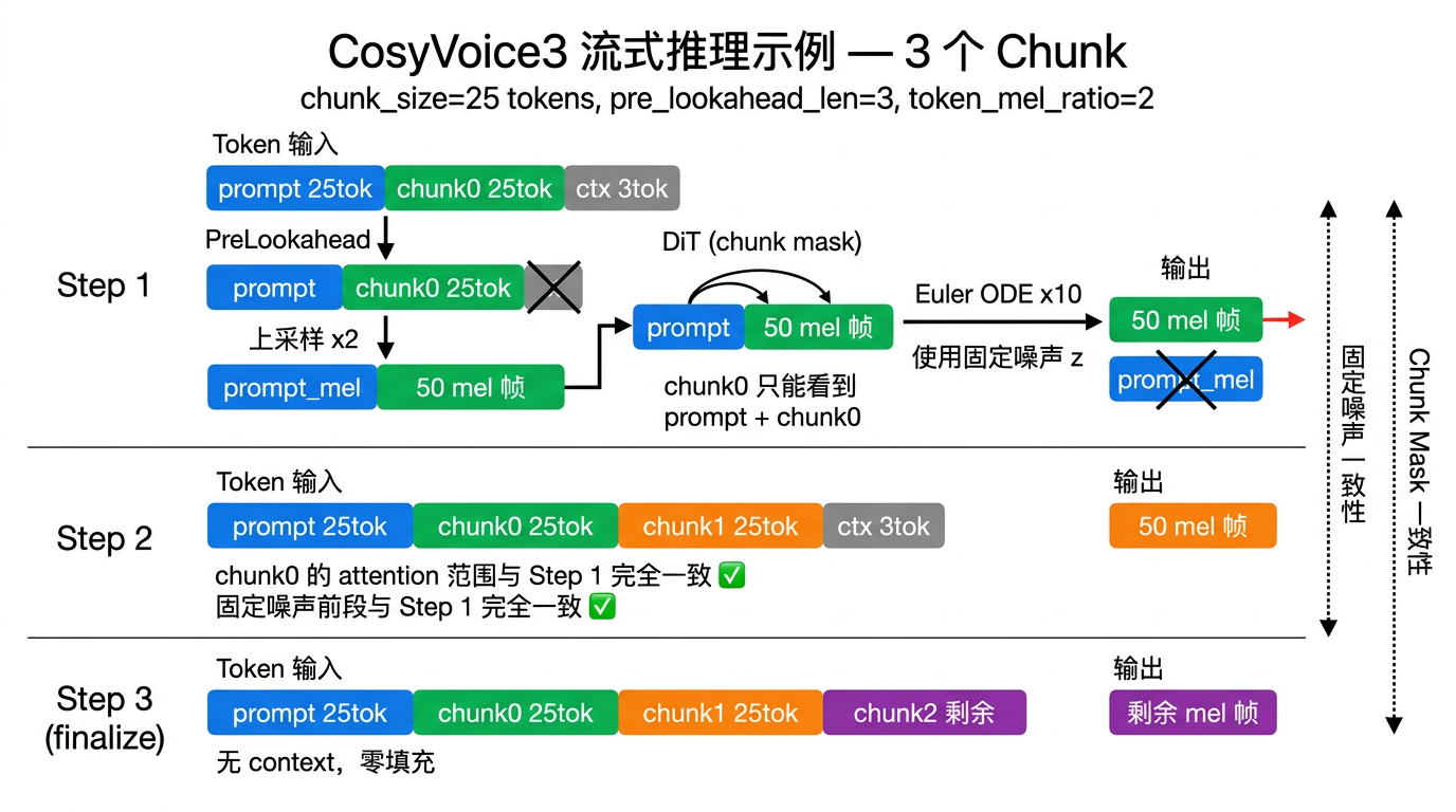
这个设计保证了流式分 chunk 推理和全序列推理的输出逐帧完全一致,具体详见第 3 章关于流式的详细解读。
2.3.2 repeat_interleave 上采样
CosyVoice3 重新设计了帧率体系,使 token 帧率和 mel 帧率为精确的 2 倍整数关系:
- token 帧率:25 Hz(
token_frame_rate=25) - mel 帧率:24000 / 480 = 50 Hz(
sample_rate=24000, hop_size=480) - 比值:
token_mel_ratio = 2
每个 token 帧重复 2 次,能够直接匹配 mel 帧率,简化模型的结构和流式设计的难点。在严格两倍关系的基础上,上采样只需一行代码:
1 | h = h.repeat_interleave(self.token_mel_ratio, dim=1) # [B, T, 80] → [B, T×2, 80] |
2.3.3 数据预处理保证帧数对齐
尽管 token 和梅尔特征的帧率在理论上是严格两倍的关系,但因为 token 和梅尔特征的提取细节存在细微差异,所以在部分特殊音频上,可能会触发两者相差1帧的问题(在语音生成任务上比较常见)。因此,为确保 token 数 × 2 == mel 帧数 严格成立,数据预处理阶段(cosyvoice/dataset/processor.py 中的 compute_fbank)会将音频长度规整到 960 的整数倍:
1 | # cosyvoice/dataset/processor.py — compute_fbank |
960 = 24000/25 = 每个 token 对应的采样点数。pad 到 960 的倍数后:
- mel 帧数 = L / 480 = 2k(偶数)
- token 数 = L / 960 = k
- token × 2 = mel 帧数,精确无误
2.4 DiT 网络
DiT(Diffusion Transformer,定义于 cosyvoice/flow/DiT/dit.py)是整个 flow matching 模块的核心。
2.4.1 模型配置参数
| 参数 | 值 | 含义 |
|---|---|---|
dim |
1024 | 隐层维度 |
depth |
22 | Transformer 层数 |
heads |
16 | 注意力头数 |
dim_head |
64 | 每头维度(16×64=1024) |
ff_mult |
2 | FFN 倍率(FFN 隐层=2048) |
mel_dim |
80 | mel 特征维度 |
mu_dim |
80 | token embedding 维度 |
spk_dim |
80 | speaker embedding 投影后维度 |
out_channels |
80 | 输出梅尔特征维度 |
static_chunk_size |
50 | 流式 chunk 大小(梅尔特征的帧数,对应1秒) |
num_decoding_left_chunks |
-1 | 默认使用全部左侧历史 |
2.4.2 模型结构与前向传播
1 | class DiT(nn.Module): |
前向传播流程:
1 | 输入: |
2.4.3 DiTBlock 细节
每层 DiTBlock 的结构(定义于 cosyvoice/flow/DiT/modules.py),实际相当于在 Transformer Encoder 的基础上增加了时间 t 影响的 AdaLN-Zero。
1 | class DiTBlock(nn.Module): |
其中,AdaLN-Zero(cosyvoice/flow/DiT/modules.py 中的 AdaLayerNormZero)是 DiT 将时间步 t 注入模型的核心机制,源自 DiT 原始论文。与标准 LayerNorm 使用固定的可学习 affine 参数不同,AdaLN-Zero 的归一化参数由时间步 t 关联生成(这种关联/影响,可以称为「调制」,类似 AdaSpeech 系列的 Conditional LayerNorm 设计思想):
1 | class AdaLayerNormZero(nn.Module): |
6 个调制向量均来自于 t 投影后的 embedding,按照作用的模块分为两组,分别用于 Attention 和 FFN 子层:
| 调制参数 | 作用位置 | 用途 |
|---|---|---|
scale_msa / shift_msa |
Attention 前 | 对 LayerNorm 输出做仿射变换:LN(x) * (1 + scale) + shift |
gate_msa |
Attention 后 | 门控 Attention 输出:x = x + gate_msa * attn_output |
scale_mlp / shift_mlp |
FFN 前 | 对 FFN 输入的 LayerNorm 做仿射变换 |
gate_mlp |
FFN 后 | 门控 FFN 输出:x = x + gate_mlp * ff_output |
设计要点:
self.norm设置elementwise_affine=False,是为了移除标准 LayerNorm 的可学习 γ/β 参数,改为完全由时间步tembedding 控制,相当于模型可以学习到不同时间t的区别- AdaLN-Zero 名称中的 “Zero”,原本意思是将
self.linear = nn.Linear(dim, dim * 6)线性层的权重初始化为零,使训练初期 DiTBlock 近似恒等映射,有利于深层网络训练稳定性(但在当前 CosyVoice 代码实现中,没有修改,nn.Linear 沿用了 PyTorch 默认的 Kaiming Uniform 初始化) - 最后一层 DiTBlock 之后使用的是
AdaLayerNormZero_Final,仅生成 scale、shift,因为后面没有 Attention 和 FFN 层了。
2.4.4 因果卷积位置编码
DiT 使用因果卷积(CausalConvPositionEmbedding)代替传统的双向卷积位置编码(均定义于 cosyvoice/flow/DiT/modules.py):
1 | class CausalConvPositionEmbedding(nn.Module): |
与非因果版 ConvPositionEmbedding(两侧 padding=15)不同,因果版只在左侧 pad 30 帧,右侧 pad 0,是严格因果的结构。每个位置仅依赖当前及之前 30 帧的信息,这是支持流式推理的基础设计。
2.5 训练目标
Flow Matching(代码位于 cosyvoice/flow/flow_matching.py)定义了一个从噪声分布
对应的目标速度场为:
模型(DiT)正是基于传入的各种条件信息,被训练来预测这个速度场
1 | # CausalConditionalCFM.compute_loss |
训练过程中,training_cfg_rate 设置 20% 概率将 mu / spks / cond 全部置零,让模型同时学习有条件和无条件分布,是 Classifier-Free Guidance(CFG)的训练配置。
2.6 推理采样
推理时,从固定噪声出发,经过 10 步 Euler ODE 求解。完整流程如下(代码位于 cosyvoice/flow/flow_matching.py):
2.6.1 Cosine 时间步调度
1 | # CausalConditionalCFM.forward |
Cosine 调度后的时间步分布:
| 步骤 | t 区间 | dt | 特点 |
|---|---|---|---|
| 1 | 0.000 → 0.025 | 0.025 | 高噪声区,小步精细去噪 |
| 2-4 | 0.025 → 0.345 | 递增 | 逐步加速 |
| 5-6 | 0.345 → 0.655 | ~0.155 | 中间阶段步长最大 |
| 7-9 | 0.655 → 0.975 | 递减 | 逐步减速 |
| 10 | 0.975 → 1.000 | 0.025 | 低噪声区,小步精细打磨 |
2.6.2 CFG 推理与 Euler 求解
每步 Euler 迭代中,构造 batch=2 同时做有条件和无条件推理,代码简写为:
1 | # 10 步 Euler 循环 |
cfg_rate=0.7 意味着对有条件预测做 1.7 倍放大、对无条件预测做 0.7 倍抑制,增强条件引导的效果。每步需要执行一次 DiT forward(batch=2 用于 CFG),10 步共 10 次 forward、20 次 DiT 计算。
以上就是 DiT 模型从输入信息到模型结构、从训练目标和推理方式的解读,结合 DiT 和 Flow Matching 相关的论文能够更方便理解。
3. 流式推理设计
CosyVoice3 DiT 最重要的参考细节是在流式的设计上,在同一个模型、同一套参数下,通过不同的 attention mask 同时支持流式和非流式推理。具体包括以下四点细节:
1 | 细节 1: Unified Training 50% 概率 streaming / 非 streaming 联合训练 |
3.1 Unified Training
1 | # CausalMaskedDiffWithDiT.forward (训练) |
训练时每个 batch 有 50% 概率使用 chunk mask、50% 使用 full mask。streaming 实际最终影响的是 DiT 的 attention mask 形状:
streaming=True:chunk mask(受限视野)streaming=False:full attention(全局视野)
3.2 Chunk Attention Mask
3.2.1 subsequent_chunk_mask
该函数定义于 cosyvoice/utils/mask.py,负责生成 chunk 级的 causal mask:
1 | def subsequent_chunk_mask(size, chunk_size, num_left_chunks=-1, device='cpu'): |
以 size=8, chunk_size=2 为例:
1 | 位置 0 1 2 3 4 5 6 7 |
可以直观地看出,chunk mask 保证的是同一 chunk 内的帧互相可见,且能看到之前所有 chunk。
3.2.2 chunk_mask 实现细节
DiT 代码中(cosyvoice/flow/DiT/dit.py),根据 streaming 标志选择不同的 mask 策略:
1 | # DiT.forward |
关键区别在于 static_chunk_size 和后续的 shape 处理:
Streaming(static_chunk_size=50):进入 add_optional_chunk_mask 的 elif static_chunk_size > 0 分支,调用 subsequent_chunk_mask(L, 50, -1) 生成 (L, L) 的 chunk 因果 mask,每个位置只能看到自身所在 chunk 及之前所有 chunk 的帧。
Non-streaming(static_chunk_size=0):进入 else 分支,直接返回 padding mask (B, 1, L)。然后通过 .repeat(1, L, 1) 扩展为 (B, L, L),每一行都是相同的 padding mask,意味着所有非 padding 位置之间双向可见,相当于全局 attention。
3.3 PreLookahead 的 context 机制
之前在 2.3 小节中提到,PreLookaheadLayer 需要看到右侧 3 帧。流式推理中,每次调用时额外传入后 3 个 token 作为 context(代码位于 cosyvoice/flow/flow.py):
1 | if finalize is True: # 最后 chunk: 无 context,pad 零(与训练一致) |
context 虽然参与了 conv1 的卷积计算,但不产生输出,这样能保证每个位置的卷积范围内容,和完整序列处理时完全一致。
3.4 固定噪声
CausalConditionalCFM(定义于 cosyvoice/flow/flow_matching.py)使用预生成的固定噪声,代替完全的随机采样:
1 | class CausalConditionalCFM(ConditionalCFM): |
固定噪声解决的问题:流式推理中会多次调用 forward,如果每次随机采样,同一个位置在不同次调用中的初始噪声不一致,是不符合 Flow Matching 的原理的。而使用固定噪声后,位置 i 的噪声永远是 rand_noise[:,:,i]。
注意:训练时使用随机噪声 torch.randn_like(x1),不需要固定,因为训练是一次处理完整序列,流式是通过 attn_mask 的设计来实现的,并不存在多次调用的一致性问题。
3.5 保证推理一致性
综合上面的信息,以下多个机制共同保证分 chunk 推理和全序列推理结果严格相等(精度误差为 0):
- PreLookahead context → 卷积输出逐位置一致
repeat_interleave→ 这一步是确定性的上采样- 固定噪声 → 每个位置的初始噪声值在不同次推理中相同
- Chunk attention mask → 每个位置的注意力范围在不同次推理中完全相同(
num_left_chunks=-1,看全部历史) - 因果卷积位置编码 → 不依赖未来,输出也逐位置一致
代码中附带了验证脚本(cosyvoice/flow/flow.py 末尾的 __main__ 块),分 chunk 推理后逐帧对比全序列推理结果,差异为 0。
3.6 流式推理的完整实现
上面 3.1~3.5 讲的是 DiT 模型层面的流式设计,本节从工程实践角度展示完整的流式推理链路:LLM 异步产 token → Flow Matching 分 chunk 生成 mel → HiFi-GAN 合成波形。代码位于 cosyvoice/cli/model.py 的 CosyVoice3Model(继承自 CosyVoice2Model)。
3.6.1 token2wav 内部细节
CosyVoice3Model 的初始化和核心方法 token2wav:
1 | class CosyVoice3Model(CosyVoice2Model): |
token2wav 的核心逻辑:
flow.inference内部已丢弃 prompt 区 mel(feat[:, :, mel_len1:]),返回全部合成区 meltoken_offset * token_mel_ratio进一步裁掉之前 chunk 已输出的部分,只留当前 chunk 新增的 mel 帧- HiFi-GAN 通过
speech_offset记录已输出的波形长度,每次只截取新增波形,这样就不需要 CosyVoice2 中的 overlap + fade-in/out 平滑拼接,因为 DiT 流式设计已保证 chunk 边界处的 mel 严格连续
3.6.2 流式 TTS 调用流程
tts 方法(继承自 CosyVoice2Model)协调 LLM 和 Flow Matching 的流水线:
1 | # CosyVoice2Model.tts —— 流式分支 |
从代码中可以看到几个关键设计:
- 等待条件 >= hop_len + pre_lookahead_len:每次送入 Flow 的 token 比实际输出多 3 个,这 3 个就是 PreLookahead 的 context(参见 3.3 节),参与卷积但不产生输出
- 首 chunk 对齐:
prompt_token_pad将 prompt token 长度向上取整到token_hop_len=25的倍数,保证 chunk 边界与 DiT 的static_chunk_size=50 mel帧对齐 - 渐进式增大 hop:
token_hop_len每次乘以stream_scale_factor=2,从 25→50→100(上限),首包用最小 chunk 降低延迟,后续用更大 chunk 提高推理吞吐 - finalize 收尾:LLM 结束后,剩余 token 不足一个 hop 时跳出循环,最后一次调用
token2wav(finalize=True)处理全部剩余 token
以 3 个 chunk 为例(chunk_size=25 token, pre_lookahead_len=3, token_mel_ratio=2),完整流程如图:
3.8 关于 Dynamic Chunk 的补充
cosyvoice/utils/mask.py 中的 add_optional_chunk_mask 函数还支持两层 dynamic 随机化(源自 WeNet 流式 ASR 框架),通过 use_dynamic_chunk 和 use_dynamic_left_chunk 两个开关分别控制。CosyVoice3 的 flow 模块未开启此模式,但是可以自己进行实验的。
3.8.1 Dynamic Chunk(动态 chunk 大小)
设置 use_dynamic_chunk=True 开启。训练时(decoding_chunk_size=0),每个 batch 随机采样 chunk 大小:
1 | chunk_size = torch.randint(1, max_len, (1,)).item() |
核心思想:模型在训练时见过各种 chunk 大小,推理时可以指定任意 decoding_chunk_size,灵活适配不同延迟需求,chunk 越大延迟越高但质量越好,chunk 越小延迟越低。
3.8.2 Dynamic Left Chunk(动态左侧历史 chunk 个数)
在 Dynamic Chunk 基础上,进一步设置 use_dynamic_left_chunk=True 开启。控制的是每个位置在 attention 中能回看多少个历史 chunk:
1 | if use_dynamic_left_chunk: |
不开启时 num_left_chunks=-1,即看全部历史。开启后,训练时随机限制可回看的历史 chunk 数量(从 0 到最大值均匀采样),推理时可以通过 num_decoding_left_chunks 指定固定值。这解决的是显存/计算量随序列增长线性膨胀的问题,限制左侧窗口后,适合超长音频的流式场景。为了保证模型效果的稳定性,训练时开启 use_dynamic_left_chunk 对于推理时限制长度理论上也是有好处的。
use_dynamic_chunk |
use_dynamic_left_chunk |
chunk 大小 | 左侧历史 | 适用场景 |
|---|---|---|---|---|
False |
False |
固定 (static_chunk_size) |
全部 (-1) |
CosyVoice3 当前方案,chunk 固定,左侧窗长持续增长 |
True |
False |
随机 [1,25] 或全序列 | 全部 (-1) |
灵活延迟,但左侧窗长持续增长 |
True |
True |
随机 [1,25] 或全序列 | 随机 [0, max] | 灵活延迟 + 控制显存 |
CosyVoice3 开源的是最简洁的方案:static chunk(固定 50 mel 帧),不做 chunk 大小或左侧窗口的动态随机化,随机性只出现在 50% 概率 streaming/non-streaming 随机切换。
4. 简要总结
CosyVoice3 的 Flow Matching + DiT 模块代表了 TTS 设计的几个趋势:
- Transformer 取代 U-Net:22 层 DiT 替代了传统 U-Net decoder,更适合序列建模且易于流式化
- 极简编码器:两层因果卷积(PreLookaheadLayer)+ repeat 上采样,模型参数更集中在 DiT 模块。
- 训练-推理一致的流式设计:通过 PreLookahead context、固定噪声、chunk mask 三者配合,实现了可靠的流式/非流式推理
- 统一训练:50% streaming / 50% non-streaming 随机切换,一套权重适配两种场景
Flow Matching / DiT 的基础原理、模型设计、流式处理,还是存在很多技术细节的,是一个生成式算法和工程设计精妙结合的典范。虽然近来 TTS 的一部分新方案在逐步去除 DiT(比如重新回到 LLM + RVQ 的思路),但其最终是否能够真正被替代还需要实践验证。
- 本文标题:代码解读 | CosyVoice 代码研读(三):CosyVoice DiT CFM
- 创建时间:2026-01-29
- 本文链接:2026/2026-01-29-cosyvoice3-dit/
- 版权声明:本博客所有文章除特别声明外,均采用 BY-NC-SA 许可协议。转载请注明出处!